2020-09-05

DS - Research - Bike accidents in Madrid

DISCLAIMER ALERT: This article is intended to be an exercise to start practicing with the Jupyter tool and Python related scientific libraries such as Pandas and Numpy. By no means it’s supposed to be considered as a reference analysis of any kind.

Bike accident analysis in Madrid city (2018-2020)

Following the Coursera course I’m in I wanted to practice with some real data out there. What best to get some insights about the city I live in ? Nowadays I normally ride my bike several days a week through the city so as you would imagine I’m very concerned about the bike accidents in the city.

The source datasets I’m using during this analysis are taken from the site Madrid council open data site. Specifically I’m using the years 2018, 2019, and 2020 (until August which is the last available dataset at the time of writing). In the resources section you can also find the Jupyter source file.

I’ve realized that conducting an analysis using a Jupyter Notebook is great not only because is one of the best tools for statistical analysis but also because I can export the notebook to asciidoc which I can convert easily to asciidoctor and copy/paste it to my blog.

Before doing any kind of analysis we need to look the data and see if we should clean it up a little bit.

2018 Dataset

Datasets before 2018 have a different formatting that datasets from 2019 and ahead. Therefore I need to make them match the rest of the datasets I’m merging it with.

*In[1]:*

import pandas as pd

def get_first_hour(hour_range_str):
    import re
    m = re.search('DE (.*) A .*', hour_range_str)
    return m.group(1)

accidents_2018 = pd.read_csv("accidents_2018.csv", delimiter=";", skiprows=0, encoding="ISO-8859-1")

accidents_2018["TIPO VEHÍCULO"] = accidents_2018["Tipo Vehiculo"]
accidents_2018["CALLE"] = accidents_2018["LUGAR ACCIDENTE"]
accidents_2018["HORA"] = accidents_2018["RANGO HORARIO"].apply(get_first_hour)

2019-2020 Datasets

Reading 2019 and 2020 CSV files.

*In[2]:*

accidents_2020 = pd.read_csv("accidents_2020.csv", delimiter=";", skiprows=0, encoding="ISO-8859-1")
accidents_2019 = pd.read_csv("accidents_2019.csv", delimiter=";", skiprows=0, encoding="ISO-8859-1")

Merging datasets 2018-2020

Finally merging all datasets into the dataframe I’ll be working with.

*In[3]:*

accidents=pd.concat([accidents_2018, accidents_2019, accidents_2020])

Preparing DataFrame to start with the analysis

Before starting with the analysis there’re a couple of steps required to make the process a little bit easier:

I’m interested only in a given set of columns:
- FECHA (Date)
- HORA (Hour)
- CALLE (Street),
- DISTRITO (District)
- TIPO VEHÍCULO (Type of Vehicle)

*In[4]:*

columns_to_keep = ["FECHA", "HORA", "CALLE", "DISTRITO", "TIPO VEHÍCULO"]
accidents = accidents[columns_to_keep].dropna()

I’m only interested in bike accidents: Ci stands for moped in spanish.

*In[5]:*

by_bike = accidents["TIPO VEHÍCULO"].str.startswith("Moto") | \
    accidents["TIPO VEHÍCULO"].str.startswith("Ci") | \
    accidents["TIPO VEHÍCULO"].str.startswith("MO")

accidents = accidents[by_bike]
accidents.drop("TIPO VEHÍCULO", axis=1, inplace=True)

I need to normalize street names:

*In[6]:*

accidents["CALLE"] = accidents["CALLE"].\
    str.replace("CALLE DE", "").\
    str.replace("CALLE", "").\
    str.replace("NUM .*", "").\
    str.replace("CALL. ", "").\
    str.replace(" - .*", "").\
    str.strip()

I need to normalize district names as well.

*In[7]:*

for x, y in [('Á', 'A'), ('Í', 'I')]:
    accidents["DISTRITO"] = accidents["DISTRITO"].\
        str.replace(x, y).\
        str.strip()

Convert string dates to actual timestamp objects

*In[8]:*

accidents["TIMESTAMP"] = accidents["FECHA"] + " " + accidents["HORA"]
accidents["TIMESTAMP"] = pd.to_datetime(accidents["TIMESTAMP"], format="%d/%m/%Y %H:%M")

Sort DataFrame by date in ascending order

*In[9]:*

accidents = accidents.sort_values("TIMESTAMP")
accidents = accidents.reset_index()
accidents.drop(["FECHA", "HORA", "index"], axis=1, inplace=True)
accidents.head()

*Out[9]:*

	CALLE	DISTRITO	TIMESTAMP
0	VIA CARPETANA	CARABANCHEL	2018-01-01 21:00:00
1	LA INFANTA MERCEDES	TETUAN	2018-01-02 12:00:00
2	LA ARMADA ESPAÑOLA	SALAMANCA	2018-01-02 13:00:00
3	EUGENIO SALAZAR	CHAMARTIN	2018-01-02 14:00:00
4	PASEO DE LA CASTELLANA	CHAMBERI	2018-01-02 15:00:00

CALLE

DISTRITO

TIMESTAMP

VIA CARPETANA

CARABANCHEL

2018-01-01 21:00:00

LA INFANTA MERCEDES

TETUAN

2018-01-02 12:00:00

LA ARMADA ESPAÑOLA

SALAMANCA

2018-01-02 13:00:00

EUGENIO SALAZAR

CHAMARTIN

2018-01-02 14:00:00

PASEO DE LA CASTELLANA

CHAMBERI

2018-01-02 15:00:00

Analysis

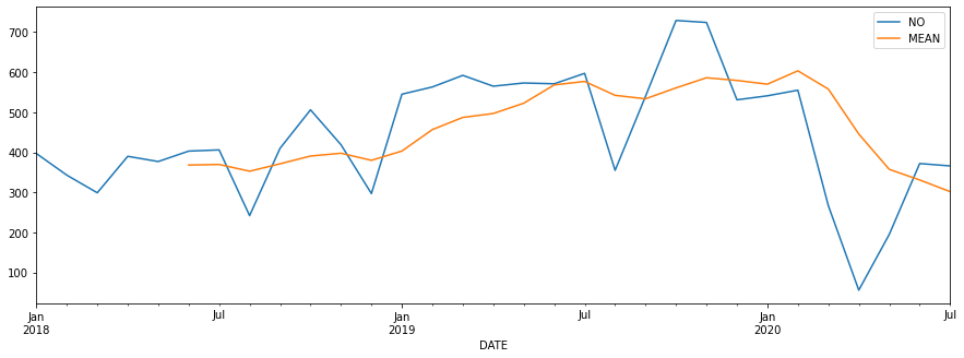
Accident trend

In this first question I’d like to address the following points:

Answer the question: Are the number of accidents increasing from 2018 ?
Show a line chart showing the trend

*In[10]:*

trends = accidents.copy()
trends["NO"] = 1
trends["MONTH"] = trends["TIMESTAMP"].dt.strftime("%m")
trends["YEAR"] = trends["TIMESTAMP"].dt.strftime("%Y")
trends = trends.set_index(["YEAR", "MONTH"])
trends = trends.groupby(["YEAR", "MONTH"]).sum()
trends = trends.reset_index()
trends["DATE"] = trends["YEAR"] + "/" + trends["MONTH"]
trends["DATE"] = pd.to_datetime(trends["DATE"], format="%Y/%m")

# getting rid of unnecessary columns
trends.drop(["YEAR", "MONTH"], axis=1, inplace=True)

# rolling mean
trends["MEAN"] = trends["NO"].rolling(6).mean()
trends = trends.set_index("DATE")

trends.plot.line(figsize=(15,5))

*Out[10]:*

Visually the first thing that sprang to mind was the huge abism on april 2020 because of the covid-19 confinement in Spain.
Despite that important fact, is also true that the general trend from 2018 was increasing significantly until october 2019. You can see the rolling mean (in yellow) going up until later 2019.

There are two patterns worth mentioning:

A decrease of accidents at holidays’ peaks (August/December)
An increase at the end of of holidays (end of August and earlier January)

You can see the increase/decrease percentage in the next dataframe.

*In[11]:*

percent = accidents.copy()

percent["NO"] = 1
percent["YEAR"] = percent["TIMESTAMP"].dt.year
percent = percent.groupby("YEAR").aggregate("sum").head()

percent = percent.reset_index()
percent = percent.rename(columns={"NO": "TOTAL"}, inplace=False)

for i in range(1, len(percent)):
    previous = percent.loc[i-1, "TOTAL"]
    current = percent.loc[i, "TOTAL"]
    percent.loc[i, "INCREMENT"] = ((current - previous) / previous) * 100

percent

*Out[11]:*

	YEAR	TOTAL	INCREMENT
0	2018	4489	NaN
1	2019	6885	53.374916
2	2020	2352	-65.838780

Worst districts by number of accidents

The worst ten district by number of accidents during these three years were:

*In[12]:*

wb = accidents.copy()
wb["NO"] = 1
wb = wb.\
    groupby("DISTRITO").\
    sum().\
    sort_values("NO", ascending=False)

wb.head(10)

*Out[12]:*

NO	DISTRITO
1517	SALAMANCA
1276	CENTRO
1264	CHAMBERI
1250	CHAMARTIN
998	TETUAN
873	CIUDAD LINEAL
776	RETIRO
699	MONCLOA-ARAVACA
648	ARGANZUELA
593	CARABANCHEL

Comparing the wost distrinct vs the best

The most dangerous district vs the safest. It turns out the district with the highest rate of accidents was the district of SALAMANCA whereas the lowest was VICALVARO. It makes sense because VICALVARO is outside the city center by far, so traffic density is also very low.

*In[13]:*

wb = wb.iloc[[0, -1]]
wb

*Out[13]:*

DISTRITO

1517

SALAMANCA

117

VICALVARO

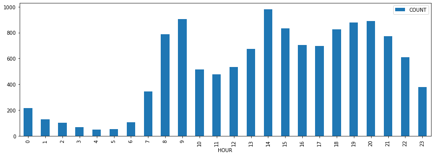
When is the best/worst hours to ride in general ?

Apart from the districts it would be nice to know which are the best/worst moment to get out there with your bike. Although we will see how rush hours are in general a bad moment to go, it seems that the worst hour to ride in general is 14h, is when most accidents occur. On the other hand, the hour with less number of accidents is 4h, which makes sense because at that hour at night you don’t see a soul on the road.

*In[14]:*

hs = accidents.copy()

hs["HOUR"] = hs["TIMESTAMP"].dt.hour
hs["DAY"] = hs["TIMESTAMP"].dt.dayofweek

hs = hs.\
    groupby(["DAY", "HOUR"]).\
    size().\
    reset_index(name="COUNT").\
    set_index("DAY")

all_week = pd.DataFrame(hs.reset_index().groupby("HOUR")["COUNT"].sum())
values = all_week.sort_values("COUNT")

worst = values.iloc[-1]
best  = values.iloc[0]

w_hour, w_no, b_hour, b_no = [worst.name, worst["COUNT"], best.name, best["COUNT"]]

message = "Best \t==> {}h  ({} accidents)\nWorst \t==> {}h ({} accidents)".format(b_hour, b_no, w_hour, w_no)
print(message)

*Out[14]:*

Best 	==> 4h  (60 accidents)
Worst 	==> 14h (1060 accidents)

Analysis of hours during the week

I’d to see visually how accidents are arrange on a working day. In order to achieve that I’m creating a bar chart with the aggregated number of accidents from Monday to Friday by hour.

*In[15]:*

week = hs.loc[0:5]
week = pd.DataFrame(week.reset_index().groupby("HOUR")["COUNT"].sum())

week.plot.bar(y="COUNT", figsize=(15,5))

*Out[15]:*

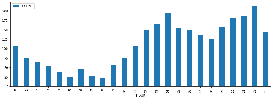
Analysis of hours during the weekend

As a biker, it’s even more important to me to analyse when is the best moment to ride my bike during the weekends. So the same way I did the analysis for the working days, here I’m doing the same for the weekend.

*In[16]:*

weekend = hs.loc[5:7]
weekend = pd.DataFrame(weekend.reset_index().groupby("HOUR")["COUNT"].sum())

weekend.plot.bar(y="COUNT", figsize=(15,5))

*Out[16]:*

Comparing week/weekend hour by hour

Fortunately the number of accidents decreases a lot during weekends, but the shape of the chart seems to be pretty similar. I’m curious to see both charts head to head to see both datasets with the same scale.

*In[17]:*

all_week = weekend.copy()
all_week["WEEK"] = week["COUNT"]

all_week.\
    rename(columns={"COUNT": "WEEKEND"}, inplace=False).\
    plot.bar(figsize=(15,5))

*Out[17]:*

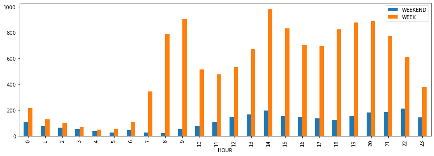
As you can see there’s a huge difference (even visually) when you compare both datasets altogether with the same scale.

Comparing weekend days hour by hour

This time I’m going directly to compare both Saturday and Sunday datasets.

*In[18]:*

saturday = hs.loc[5]
saturday = pd.DataFrame(saturday.reset_index().groupby("HOUR")["COUNT"].sum()).\
    rename(columns={"COUNT": "SATURDAY"})

sunday = hs.loc[6]
sunday = pd.DataFrame(sunday.reset_index().groupby("HOUR")["COUNT"].sum()).\
    rename(columns={"COUNT": "SUNDAY"})

pd.merge(saturday, sunday, how="inner", on="HOUR").\
    plot.bar(figsize=(15,5))

*Out[18]:*

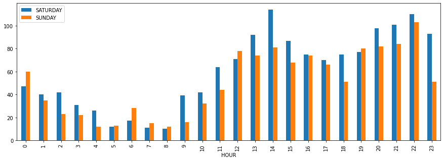
I can observe that in general, there’re more accidents during Satuday than Sunday. The exception is the earlier hours on Sunday which I guess corresponds people hanging out and at sunset on Sunday when these people are coming home and some other people are heading work (e.g: bakers).

Blackspots: Streets with highest rate of aggregated accidents

Which are the streets with the highest number of accidents overtime ?

*In[19]:*

bs = accidents.copy()
bs.groupby(["CALLE", "DISTRITO"]).\
    size().\
    reset_index(name='COUNT').\
    sort_values("COUNT", ascending=False).\
    head(10).\
    reset_index().\
    drop("index", axis=1)

*Out[19]:*

	CALLE	DISTRITO	COUNT
0	BRAVO MURILLO	TETUAN	145
1	ALCALA	SALAMANCA	123
2	ALCALA	CIUDAD LINEAL	123
3	SERRANO	SALAMANCA	80
4	GRAN VIA	CENTRO	72
5	ARTURO SORIA	CIUDAD LINEAL	72
6	PASEO. CASTELLANA	CHAMARTIN	60
7	FRANCISCO SILVELA	SALAMANCA	58
8	PASEO. CASTELLANA	TETUAN	57
9	JOAQUIN COSTA	CHAMARTIN	56

I can see a clear winner with the BRAVO MURILLO street, followed by ALCALA. Alcala makes sense to me because it’s a really long street spanning different districts, so it’s naturally busy all the time. But I have to admit that I wouldn’t have said Bravo Murillo, not in a million years.

Next steps

I’d like to create a probability table in order to answer the question: What is the probability of having an accident at a given district at a given day of the week at a given hour ? That requires some missing numbers I have to get before going any further.