2020-11-13

Linear Regression notes

Classification is a great method to predict discrete values from a given dataset, but sometimes you need to predict a continuous value, e.g: height, weight, prices… And that’s when linear regression techniques come handy.

What is linear regression ?

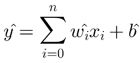
The definition that I read in the Wikipedia didn’t help me at all. Instead when I related it with a line, it started to make sense to me. If we’ve got a linear function, that is, a function describing a line, where ŵ is the slope of the line and b is called the intercept which is a constant value:

Figure 1. linear function

For every x value a new point will be drawn and eventually altogether will form a line. So, if you think about it visually, given a set of input values, a simple linear regression algorithm will try to come up with a line trying to pass as close as possible to the majority of the input dataset points. So if you try to predict an output value from the input values, the machine learning process will pick up a value from that line.

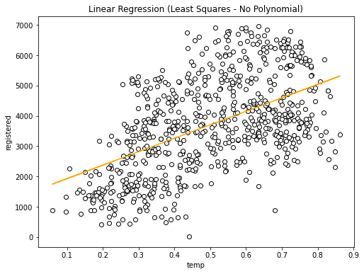
Figure 2. Simple linear regression

There’re differences between the types of linear regression techniques depending on the presence of regularization (Ridge and Lasso), or the lack of it (Simple Linear Regression). There’s also important the use of polynomial transformation and normalization.

Simple Linear Regression

The most popular linear regression uses the least squares technique. It tries to find a slope (w) and constant value (b) that minimizes the mean squared error of the model. It doesn’t have parameters to control model complexity, everything it needs is estimated from training data.

Although it could be easier, I didn’t want to made up a dataset to practice, because one of the things I’m finding most difficult while learning machine learning is to extrapolate simple examples to real world problems. I also tried to use several public datasets out there that I thought they could match well with a regression solution, but in the end and after having a dismal failure trying to make it work I had to gave up and use a specific dataset prepared for regression. The actual dataset used for this entry is a Bike sharing dataset from the UCI Dataset repository for machine learning.

I’m loading the Bike sharing daily dataset:

reading daily rental data

import pandas as pd
from datetime import datetime, date

bikes = pd.read_csv("day.csv", parse_dates=['dteday'])
bikes.head()

First, I’d like to see how features could be related to each other using the seaborn’s correlation heatmap:

creating correlation table

import numpy as np
import matplotlib.pyplot as plt
import seaborn as sns

# use all columns except the date column
bikes = bikes.loc[:, bikes.columns != 'dteday']
corr  = np.corrcoef(bikes.T)

plt.figure(figsize=(10, 10))
sns.heatmap(
    corr,
    cbar=False,
    annot=True,
    yticklabels=bikes.columns,
    xticklabels=bikes.columns)
plt.show()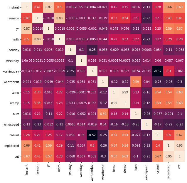

Figure 3. correlation table

There are a lot of features, but I’m focusing on just choosing one, temp which is the normalized temperature in Celsius the day of the rental. I’d like to see how it looks like visually the relationship between registered number of rentals (registered variable) and the temperature feature I’ve chosen:

pair plot

import seaborn as sns

sns.pairplot(bikes[['temp', 'registered']])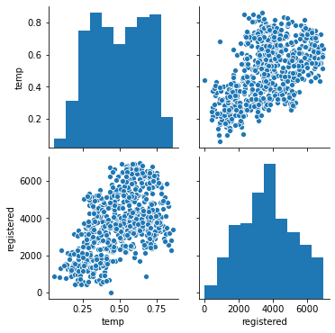

Figure 4. pair plot

What I’m looking for at this point in the scatter plot, is tendencies. In this case it seems that points tend to go in diagonal from the bottom left to the upper right part of the graph. So far, the more tendency I see the better it seems to work. Now lets create a linear regression using the LinearRegression class from scikit-learn:

creating a simple linear regression

from sklearn.linear_model import LinearRegression
from sklearn.model_selection import train_test_split

feats = ['temp']
label = 'registered'

X = bikes[feats]
y = bikes[label]

X_train, X_test, y_train, y_test = train_test_split(X, y, random_state=0)

linear_reg  = LinearRegression().fit(X_train, y_train)
score_train = linear_reg.score(X_train, y_train)
score_test  = linear_reg.score(X_test, y_test)

print("train: {}, test: {}".format(score_train, score_test))

scores

train: 0.2894397189330029, test: 0.29427542275712537

If we draw the regression line we’ve got:

regression line

import matplotlib.pyplot as plt

y_predict = linear_reg.predict(X_test)

plt.figure(figsize=(8, 8))
plt.title("Linear Regression (Least Squares - No Polynomial)")
plt.xlabel('temp')
plt.ylabel('registered')
plt.scatter(X['temp'], y, edgecolor='black', color='w')
plt.plot(X_test, y_predict, color='orange')
plt.show()

Figure 5. regression line

As you can see a straight line won’t be able to do good predictions. A way of helping the linear transformation to adapt better to the shape of the model is to use a polynomial transformation.

Polynomial Transformation

When the problem doesn’t fit easily a straight line or there are many features, it could become complicated to find a good relationship between them, specially with a simple line. The polynomial transformation helps finding those relationships. Applying a polynomial transformation to our problem can help the linear regression to adapt better to the shape of the data. This is the same linear regression example, but this time applying the PolynomialFeatures class prior to the linear regression fit.

applying polynomial transformation

from sklearn.linear_model import LinearRegression
from sklearn.model_selection import train_test_split
from sklearn.preprocessing import PolynomialFeatures

feats = ['temp']
label = 'registered'

X = bikes[feats]
y = bikes[label]

degrees = 3
X_poly  = PolynomialFeatures(degree=degrees).fit_transform(X)

X_train, X_test, y_train, y_test = train_test_split(X_poly, y, random_state=0)

linear_reg  = LinearRegression().fit(X_train, y_train)
score_train = linear_reg.score(X_train, y_train)
score_test  = linear_reg.score(X_test, y_test)

print("train: {}, test: {}".format(score_train, score_test))

scores

train: 0.3427117865309586, test: 0.371685603196769

Because the polynomial transformation is creating more features, they cover a wider spectrum of the data, therefore more likely to do better predictions, at least in the training dataset. If we draw now the result:

import matplotlib.pyplot as plt

y_predict = linear_reg.predict(X_test)

plt.figure(figsize=(8, 6))
plt.title("Linear Regression (Least Squares - Polynomial)")
plt.xlabel('temp')
plt.ylabel('registered')
plt.scatter(X['temp'], y, edgecolor='black', color='w')

colors = {1: 'orange', 2: 'green', 3: 'red'}

# drawing each new feature derived from the initial temp feature
for i in range(1, degrees + 1):
    plt.plot(X_test[:,i], y_predict, color=colors[i], alpha=0.6)

plt.show()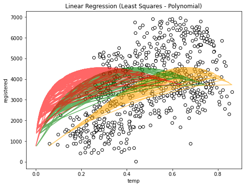

Figure 6. polynomial regression

Which covers much more than the previous example. However there are a couple of things to keep in mind when applying the polynomial transformation:

Polynomial transformation with a high degree value could overfit the model
It’s better to combine it with a regularized regression method like Ridge.

Resources

Regularization and Normalization

Regularization

Regularization is a technique used to reduce the model complexity and thus it helps dealing with overfitting:

It reduces the model size by shrinking the number of parameters the model has to learn
It adds weight to the values so that it tries to favor smaller values

Regularization penalizes certain values by using a loss function with a cost. This cost could be of type:

L1: The cost is proportional to the absolute value of the weight coefficients (Lasso)
L2: The cost is proportional to the square of the value of the weight coefficients (Ridge)

Regularization really shines when there is a high dimensionality, meaning there’re multiple features. So in these examples it won’t make a huge impact with the scores.

Normalization

Data normalization is the process of rescaling one or more features to a common scale. It’s normally used when features used to create the model have different scales. There are a few advantages of using normalization is such scenario:

It could improve the numerical stability of your model
It could speed up the training process

Normalization is specially important when applying certain regression techniques, as regression is sensitive to model feature adjustements.

Because in this article I’m only using ONE feature, normalization is not going to make much difference but, when using multiple features, and each of them in different scales, then we should use normalization.

Resources

Ridge

Follows the leat-squares criterion but it uses regularization as a penalty for large variations in w parameters.
Regularization prevents overfitting by restricting the model, it normally reduces its complexity
Regularization is controlled by the alpha parameter
The high the value of alpha the simpler the model, that is, the model is less likely to overfit

Now I’m using Ridge class with the same dataset:

using Ridge regression

from sklearn.linear_model import Ridge
from sklearn.model_selection import train_test_split

X_train, X_test, y_train, y_test = train_test_split(X, y, random_state=0)

ridge = Ridge(alpha=20).fit(X_train, y_train)

score_train = ridge.score(X_train, y_train)
score_test = ridge.score(X_test, y_test)

print("train: {}, test: {}".format(score_train, score_test))

Giving me the following scores:

train: 0.21131995467057785, test: 0.19818161857049388

Although it seems worst than the polynomial example, the takeaway idea here is that the Ridge regression along with a high value of alpha is going to reduce the complexity of the model and make the generalization more estable.

Ridge regression score can be improved by applying normalization to the source dataset. Is important for some ML methods that all features are on the same scale. In this case we’re apply a MinMax normalization.

Ridge with scaled set

from sklearn.linear_model import Ridge
from sklearn.preprocessing import MinMaxScaler
from sklearn.model_selection import train_test_split

X_train, X_test, y_train, y_test = train_test_split(X, y, random_state=0)

scaler         = MinMaxScaler()
X_train_scaled = scaler.fit_transform(X_train) # fit with the X_train
X_test_scaled  = scaler.transform(X_test)      # apply THE SAME scaler

ridge = Ridge(alpha=20).fit(X_train_scaled, y_train)

score_train = ridge.score(X_train_scaled, y_train)
score_test  = ridge.score(X_test_scaled, y_test)

print("train: {}, test: {}".format(score_train, score_test))

scores

train: 0.24767875041471266, test: 0.23615269197631883

We can use the scaled X to train the Ridge regression. However there’re some basic tips to be aware of:

Fit the scaler with the training set and then apply the same scaler to transform the training and test feature sets
Don’t use the test dataset to fit the scaler. That could lead to data leakage.

Lasso

It uses a L1 type regularization penalty, meaning it minimizes the sum of the absolute values of the coefficients
It works as a kind of feature selection
It also has an alpha parameter to control regularization

using lasso regression

from sklearn.linear_model import Ridge, Lasso

lasso = Lasso(alpha=20).fit(X_train, y_train)

score_train = lasso.score(X_train, y_train)
score_test = lasso.score(X_test, y_test)

print("train: {}, test: {}".format(score_train, score_test))

scores

train: 0.2842911095363777, test: 0.2813866438355652

And finally using MinMaxScaler to try to improve regression scoring:

lasso with scaled features

from sklearn.preprocessing import MinMaxScaler
from sklearn.linear_model import Ridge, Lasso
from sklearn.model_selection import train_test_split

X_train, X_test, y_train, y_test = train_test_split(X, y, random_state=0)

scaler         = MinMaxScaler()
X_train_scaled = scaler.fit_transform(X_train)
X_test_scaled  = scaler.transform(X_test)

lasso = Lasso(alpha=20).fit(X_train_scaled, y_train)

score_train = lasso.score(X_train_scaled, y_train)
score_test  = lasso.score(X_test_scaled, y_test)

print("train: {}, test: {}".format(score_train, score_test))

scores

train: 0.2865231606947747, test: 0.285332265748411

Results Summary

Finally I’ve written a summary table.

Table 1. Results summary
TYPE	SCIKIT CLASS	POLYNOMIAL	NORMALIZATION	REGULARIZATION	TRAIN SCORE	TEST SCORE
Linear	LinearRegression	No	No	No	0.2894397189330029	0.29427542275712537
Linear	LinearRegression	Yes	No	No	0.3427117865309586	0.371685603196769
Ridge	Ridge	Yes	No	Yes	0.21131995467057785	0.19818161857049388
Ridge	Ridge	No	Yes	Yes	0.24767875041471266	0.23615269197631883
Lasso	Lasso	No	No	Yes	0.2842911095363777	0.2813866438355652
Lasso	Lasso	No	Yes	Yes	0.2865231606947747	0.285332265748411

Lasso as feature selection method

So far I’ve been working with just one feature temp to predict a possible outcome. I chose this feature by using the correlation table as a guide. When looking for just one variable to work with, it could be enough, but when looking for many possible features it could be cumbersome. The Lasso regression seems a better method for telling me which features do perform and which don’t. How ? Well according to how the L1 regulation method works, keeping it short, those features that are not so important, Lasso makes its coefficient equal to 0, therefore, those features having a coefficient greater than 0 are worth using them to train the model (the higher the better). Lets use this knowledge to know which features could be useful to train the model.

using all possible features to see which one fits best in case we only want to use one

from sklearn.preprocessing import MinMaxScaler
from sklearn.linear_model import Ridge, Lasso
from sklearn.model_selection import train_test_split

all_features = list(bikes.columns.values)

# removing all not feature suitable columns (dteday was already removed)
all_features.remove('registered')
all_features.remove('casual')
all_features.remove('cnt')

# then doing the regression with all the remaining features
X            = bikes[all_features]
y            = bikes['registered']

X_train, X_test, y_train, y_test = train_test_split(X, y, random_state=0)

lasso       = Lasso(alpha=20).fit(X_train, y_train)

# showing features with their coefficients
feats_coeff = dict(zip(all_features, lasso.coef_))
feats_coeff

Which shows the following map:

features along with their coefficients

{'instant': 4.6922455121283315,
 'season': 403.43794430245987,
 'yr': 0.0,
 'mnth': -147.25674152072335,
 'holiday': -0.0,
 'weekday': 40.46762455840893,
 'workingday': 830.067983219723,
 'weathersit': -506.75253043165566,
 'temp': 2732.6155708939527,
 'atemp': 0.0,
 'hum': -0.0,
 'windspeed': -0.0}

Now as the theory stated, we can discard those features with 0 value, and maybe those which are negatively correlated. For this example, where I’m only interested in one feature to validate whether I chose the most significant feature or not. In this case I’m getting the feature with the highest possitive coefficient:

from sklearn.preprocessing import MinMaxScaler
from sklearn.linear_model import Ridge, Lasso
from sklearn.model_selection import train_test_split

# getting only the NON ZERO features
best_features = {k:v for (k, v) in sorted(feats_coeff.items(), key=lambda x: -x[1]) if v > 0}

# getting the higher ranked
best_feature = list(best_features.keys())[0]
best_feature

'temp'

Nice!

Ridge vs Lasso

In this case we’ve used both algorithms with the same dataset, but there’re situations where one or the other fit best:

Ridge: Many small/medium sized effects
Lasso: Few medium/large sized effects