2021-04-24

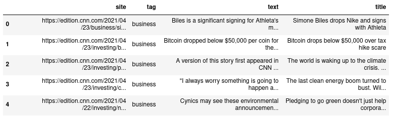
NLP: Classifying Business News

In this article I’ve collected different news from different online newspapers. These news are about politics, business, sports and general news about the world. The idea is to train a binary classifier to decide whether a given article is about business or not.

Preparing data

First of all I would like to load the xml source files and create a Pandas DataFrame. For traversing the document’s xml I’m using the ElementTree API.

loading xml files and create a DataFrame

import numpy as np
import pandas as pd
import xml.etree.ElementTree as ET

from os import walk

# all files are in the news directory
_, _, filenames = next(walk('news'))
df       = pd.DataFrame()

for file in filenames:
    xml = ET.parse("news/" + file).getroot()
    for entry in xml.findall('entry'):
        title= entry.find("title").text
        text = entry.find("text").text
        site = entry.find("link").text
        tag  = entry.find("tag").text

        df = df.append({"title": title, "text": text, "tag": tag, "site": site}, ignore_index=True)

df.head()

Creating labels

Because this is a binary classification, I need to create a column with the instances' labels. I’m creating column "business" with possible values 0 or 1 .Business related news will have 1, and the rest 0. I’m making use of Numpy’s where function.

df = df\
    .fillna({"tag": "unknown"})\
    .dropna()

df['business'] = np.where(df['tag'] == 'business', 1, 0)

Checking class imbalance

Class imbalance is an important issue. If there’are many more instances of one class than the other, the model could end up performing as if it were a dummy classifier taking the most frequent outcome as prediction. To address that problem there’re some techniques to apply like under-sampling or over-sampling. But first, lets see if there’s a clear imbalance between our two classes:

Checking class imbalance

df.loc[:, ['title', 'business']]\
    .groupby('business')\
    .count()\
    .reset_index()\
    .rename(columns={'title': 'count'})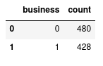

It seems there’s nothing to worry about, both classes are around 50% (52/47).

Avoid data leakage

Another important issue when dealing with data is data leakage (Wikipedia). Leaking information while training the model could create over-optimistic models that generalize badly. I’ve found some data I need to remove from text before training the model: site name and topic name.

Of course there could be more potential data leakages, for example, leaving article authors, could be a potential data leakage if those journalists are only specialized in a specific topic. For this exercise I stopped looking for data leakages when the different model predictions were performing decently with the testing datasets. There’s a very interesting article regarding data leakage that I’d like to review when I have the time.

Removing site information

Lets say an article is from the Financial Times and inside the text there is www.ft.com. Because most articles from Financial Times are supposed to be about businesses, the model could immediately correlate the site with the business class, creating overfitted models. Therefore I had to extract the different site names from the articles' links (site column in the data-frame):

getting different site names

sites = df['site']\
    .str.extractall(r'https://.*\.(?P<www>\w*)\..*')\
    .reset_index(col_fill='origin')['www']\
    .unique()

sites

[bbc, cnn, cnbc, investing...]

Once I had the site names, it was time to remove all these names from text, whether they were found as upper, lower or capitalize case.

removing site related information

for site in sites:
    df['text'] = df['text'].str.replace(site, ' ', regex=False)
    df['text'] = df['text'].str.replace(site.upper(), ' ', regex=False)
    df['text'] = df['text'].str.replace(site.capitalize(), ' ', regex=False)

Removing topic words in text

If the training text has the section it belongs: business, sports… etc, that could end up ending in a bad generalization as well.

removing topic words

for topic in ['business', 'sport', 'politics', 'investing']:
    df['text'] = df['text'].str.replace(topic, ' ', regex=False)
    df['text'] = df['text'].str.replace(topic.upper(), ' ', regex=False)
    df['text'] = df['text'].str.replace(topic.capitalize(), ' ', regex=False)

Removing stopwords

Stopwords are everywhere in text, and most of the time, they only add noise to the model, and makes training longer, so it’s better to get rid of them.

removing stopwords

from nltk.corpus import stopwords

for sw in stopwords.words('english'):
    df['text'] = df['text'].str.replace("\s{}\s".format(sw), ' ', regex=True)
    df['text'] = df['text'].str.replace("\s{}\s".format(sw.upper()), ' ', regex=True)
    df['text'] = df['text'].str.replace("{}\s".format(sw.capitalize()), ' ', regex=True)

Training model

Once I’ve finished preparing the data, it’s time to create the model.

Splitting data

First lets split the initial dataset to create training and testing datasets.

from sklearn.model_selection import train_test_split

X_train, X_test, y_train, y_test = train_test_split(df['text'], df['business'], random_state=0)

Vectorizing data sets

Unfortunately classifiers don’t deal well with categorical data such text, that’s why I’m going to use a vectorizer. According to the Scikit-Learn site Vectorization is the general process of turning a collection of text documents into numerical feature vectors. There are a few different vectorizers available in Scikit-Learn: CountVectorizer and TfidfVectorizer. In this case I’m using CountVectorizer.

from sklearn.feature_extraction.text import CountVectorizer

vec = CountVectorizer(min_df=8, ngram_range=(1,2)).fit(X_train)

print("no of features:", len(vec.get_feature_names()))

no of features: 6551

There are a couple of parameters woth commenting:

min_df: I’d like to ignore terms don’t appearing in at least in 8 documents
ngram_range: I’d like the vectorizer to create means unigrams (1, 1) and bigrams (1, 2).

ngrams

A n-gram is a sequence of phonems where n could be any positive number. That allows our comparison procedure to be smarter. Instead of comparing all characters, or word by word, in this case, we would like to find certain tuples of common tokens between two sentences. For example, What are the n-grams of sentence_1, with n=2 using tokens ?

import nltk
from nltk.util import ngrams

seq_1 = set(nltk.word_tokenize("I am a big fan"))
seq_2 = set(nltk.word_tokenize("I am a tennis fan"))

list(ngrams(seq_1, n=2)), list(ngrams(seq_2, n=2))

n-grams

([('am', 'fan'), ('fan', 'big'), ('big', 'I'), ('I', 'a')],
 [('am', 'tennis'), ('tennis', 'fan'), ('fan', 'I'), ('I', 'a')])

Once the vectorizer has been trained I can create my vectorized versions of X_train and X_test features.

transforming datasets

X_train_vectorized = vec.transform(X_train)
X_test_vectorized  = vec.transform(X_test)

Cross Validation

To figure out which classifier works best with the data at hand, I’m going to make use of cross validation to train three different classifiers.

classifiers to use

from sklearn.svm import SVC
from sklearn.ensemble import AdaBoostClassifier
from sklearn.linear_model import LogisticRegression

classifiers = [
    {
        'classifier': SVC(),
        'params': {
            'C': [1, 5, 10, 20, 30, 40],
            'kernel': ['rbf', 'linear']
        }
    },
    {
        'classifier': LogisticRegression(),
        'params': {
            'C': [1, 5, 10, 20, 30, 40],
            'solver': ['newton-cg', 'saga']
        }
    },
    {
        'classifier': AdaBoostClassifier(),
        'params': {
            'n_estimators': [50, 60, 75, 100]
        }
    }
]

I’ve created the following function that uses GridSearchCV to look for the best params to use for a given dataset.

function to get best parameters

from sklearn.model_selection import GridSearchCV
from sklearn.metrics import confusion_matrix

def resolve_best_params(classifier_entry, X_param, y_param):
    clsf_instance = classifier_entry['classifier']
    clsf_params   = classifier_entry['params']
    grid_search   = GridSearchCV(
        clsf_instance,
        cv=5,
        param_grid=clsf_params,
        scoring='precision_macro')
    grid_result   = grid_search.fit(X_param, y_param)

    return grid_result.best_params_

For every classifier I’m using resolve_best_params to find the best params for every one of them. I’m storing that information in the classifier’s dictionary to use it later.

for clsf in classifiers:
    best_params = resolve_best_params(clsf, X_train_vectorized, y_train)
    classifier  = clsf['classifier'].set_params(**best_params).fit(X_train_vectorized, y_train)
    clsf_name   = type(classifier).__name__

    # storing information for later use
    clsf['predicted']   = classifier.predict(X_test_vectorized)
    clsf['matrix']      = confusion_matrix(y_test, clsf['predicted'])
    clsf['best_params'] = best_params

Evaluation

After training different models, it’s time to see which one performs best.

Confusion Matrix

The first evaluation method I’d like to use is a confusion matrix. That will give me an idea of the precision/recall relationship for each one of them.

import seaborn as sns
import matplotlib.pyplot as plt

f, ax = plt.subplots(1, 3, figsize=(15, 5))
cols  = 0

for clsf in classifiers:
    clsf_name   = type(clsf['classifier']).__name__
    matrix      = clsf['matrix']

    ax[cols].title.set_text(clsf_name)
    sns.heatmap(matrix, cbar=False, square=True, annot=True, fmt='g',ax=ax[cols],cmap="YlGnBu")
    cols += 1

plt.show()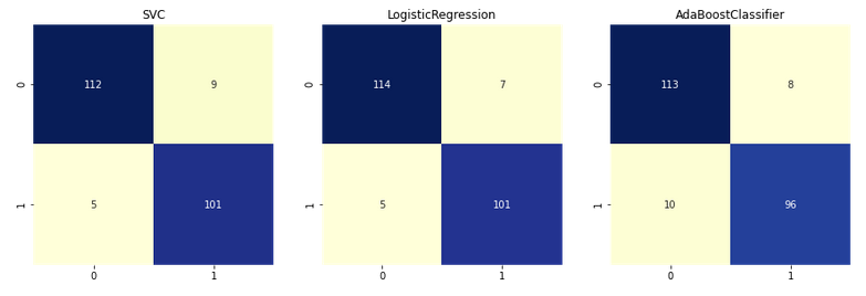

It seems that the best classifier is the one using LogicRegression.

AUC

To establish the goodness of classifier is oftenly used as a mesure the AUC or Area Under the Curve.

import matplotlib.pyplot as plt
from sklearn.metrics import roc_curve, auc

f, ax = plt.subplots(1, 3, figsize=(15, 5))
cols  = 0

for clsf in classifiers:
    clsf_name   = type(clsf['classifier']).__name__

    y_test_predicted     = clsf['predicted']
    fpr, tpr, thresholds = roc_curve(y_test, y_test_predicted)
    roc_auc              = auc(fpr, tpr)

    ax[cols].title.set_text("{0} -- AUC: {1:.2f}".format(clsf_name, roc_auc))
    ax[cols].set_xlabel("False Positive Rate")
    ax[cols].set_ylabel("True Positive Rate")
    ax[cols].plot(fpr, tpr, c='k')
    ax[cols].plot([0, 1], [0, 1], c='k', linestyle='--')
    ax[cols].fill_between(fpr, tpr, hatch='\\', color='none', edgecolor='#cccccc')
    cols +=1

plt.show()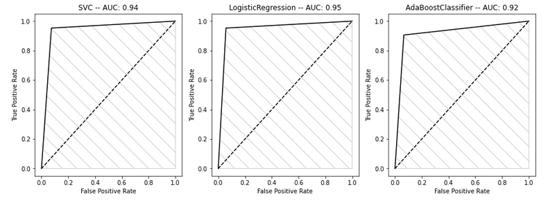

Again, it seems the classifier that is performing the best is the LogisticRegression classifier.

WordCloud

Now that it seems that the best classifier to use is LogisticRegression, I’d like to see which features are used the most when classifying a new instance as 'business'. In order to do that I’m extracting LogisticRegression’s feature coeficients.

First thing to do, I need to get the best parameters for the LogisticRegression classifier found during the cross validation I did earlier.

for clsf in classifiers:
    name   = type(clsf['classifier']).__name__
    params = clsf['best_params']
    print(name, params)

SVC {'C': 20, 'kernel': 'rbf'}
LogisticRegression {'C': 5, 'solver': 'newton-cg'}
AdaBoostClassifier {'n_estimators': 75}

Then I’m creating two groups: less and most significant features

feature_names     = np.array(vec.get_feature_names())
model             = LogisticRegression(C=5, solver='newton-cg').fit(X_train_vectorized, y_train)
sorted_coef_index = model.coef_[0].argsort()

less = feature_names[sorted_coef_index[:50]]
most = feature_names[sorted_coef_index[:-51:-1]]

And finally I’m using the WordCloud library to show a word cloud showing the most significant features and another showing the less significant features.

import matplotlib.pyplot as plt
from wordcloud import WordCloud

less_cloud = WordCloud(max_font_size=50, max_words=100, background_color="white").generate(" ".join(less))
most_cloud = WordCloud(max_font_size=50, max_words=100, background_color="white").generate(" ".join(most))

_, ax = plt.subplots(1, 2, figsize=(15, 15))

ax[0].set_title("MOST SIGNIFICANT WORDS")
ax[0].imshow(most_cloud, interpolation="bilinear")
ax[0].axis("off")

ax[1].set_title("LESS SIGNIFICANT WORDS")
ax[1].imshow(less_cloud, interpolation="bilinear")
ax[1].axis("off")

plt.show()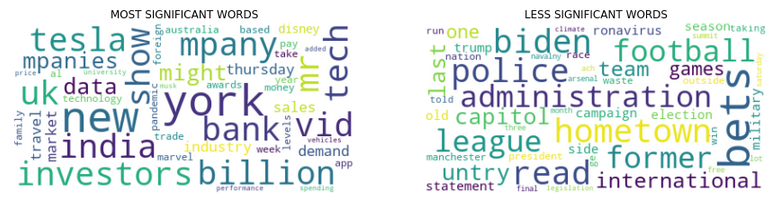

Lets use the created model to classify new instances:

predicting

news = [
    "The last Roaring Twenties ended in disaster. Should investors be worried?",
    "Bunny attends baseball game and everyone is in love with it"
]

model.predict(vec.transform(news))

Which outputs the expected results: 1 for the first text (busines) and 0 for the second text (not business):

[1, 0]

Conclusion

Wrapping up. These are the steps I followed:

Data cleaning: loading, cleaning, data leakage removal
Training model: splitting data, vectorization, cross validation to look for best parametrization
Evaluation: confusion matrix, area under the curve
Testing model with new instances

Things I could have done better:

I didn’t keep some data apart from the beginning
I didn’t create a baseline to compare the performance of the real classifiers

Resources

Data Leakage definition: Wikipedia
Data leakage article: at machinelearningmastery.com
Stopwords in NLP
Text Feature Extraction in Scikit-Learn
Wordcloud: Python library to create word clouds